Pretty fitting that we have our article on circular column capacity on pi day (March 14th) :P. We’re picking back up right where we left off from Part 1 (rectangular column/drilled shaft capacity), and are ready to approach calculating PM capacities for a circular cross-section. The big (and fun) issue here is: how are we going to find the area and the centroid of the compression block?

Assumptions
Here’s a quick reminder on the assumptions listed in part 1. These are either required or allowed by AASHTO section 5.6.2.
- Strain compatibility - plane sections remain plane, reinforcement is fully developed and bonded, and strain is directly proportional to distance from the neutral axis.
- Maximum usable concrete compressive strain is 0.003.
- Elastic perfectly plastic steel reinforcement stress-strain relationship.
- Concrete tensile strength is neglected.
- Rectangular compressive stress distribution assumed for strength limit state for concrete (Whitney stress block).
- Concrete strength is less than or equal to 10 ksi.
- Reinforcing steel yield strength is less than or equal to 100 ksi.
- AASHTO compression-controlled vs. tension-controlled strain limits used to calculate phi factors.
In this article, we will begin including the compression reinforcement in our calculation.
As stated in the assumptions we will be assuming a rectangular compressive stress distribution as outlined in AASHTO (based on Whitney stress block). This is pretty clearly allowed by AASHTO, but I was interested if the results would be as good as they are in the case of a rectangular cross-section. Multiplying the depth of the stress block by 0.85 seems like it might do something a little different when the compression area is a circular segment rather than a rectangle.
We will proceed ahead with this assumption though, as integrating a parabolic, or any other, compressive stress distribution over the area of a circular segment, finding both the volume and the centroid, is exceedingly difficult. I’m not positive that a closed-form solution is impossible, but I think it is. So it would require numerical integration, which is a lot less fun. We’ll compare our results to SpColumn’s results in Part 3, and see how the rectangular distribution assumption stacks up against a more precise one.
Segment Area Derivation
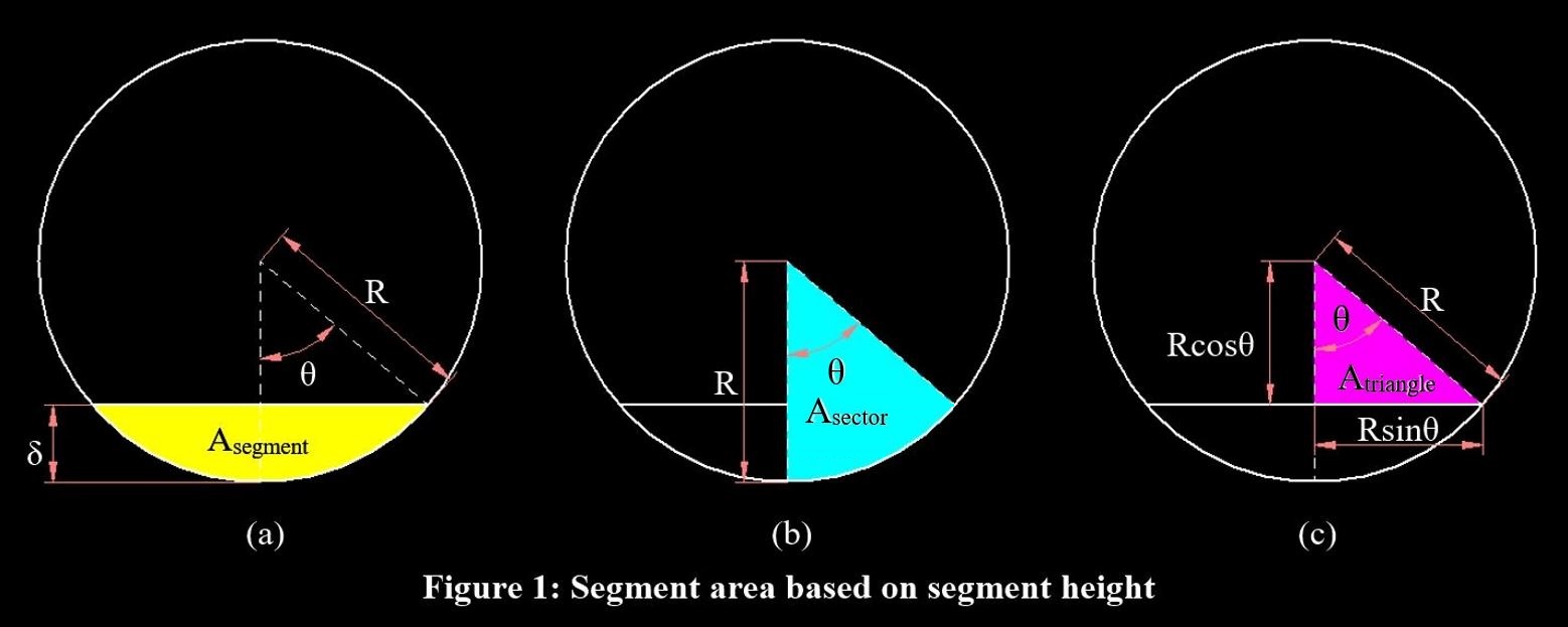
First, we have to relate the depth of the assumed compression block to the area of said block. This requires creating a formula for the area of a circular segment based on its depth. To do so, I created the figures below.
Deriving these formulas will take a good bit of trigonometry and calculus. Fortunately I figured out how to solve these back in 2014 when I first took a stab at making this type of calculator, and I had my notes saved in a word file on Dropbox. Pretty cool to see!
I’m grateful, because calculus must have been much fresher on my mind back then, and it would have taken me ages to figure this out from scratch today. But hopefully I can demonstrate the steps slowly and clearly.
As can be seen in Figure 1a, we are seeking to calculate \(A_{segment}\), using only the variables of segment depth, \(\delta\) and radius, \(R\). We will begin by relating \(\delta\) to the associated interior angle \(\theta\) as can be seen in Figure 1c.
\[\delta = R-Rcos(\theta) \tag{1}\]
Next we will relate the segment area to the sector area (the whole light blue slice of the pie in Figure 1b) and the triangle area.
\[A_{segment}/2 = A_{sector}-A_{triangle}\]
And now we put that equation in terms of \(R\) and \(\theta\).
\[A_{sector} = \frac{\theta}{2\pi}({\pi}R^2) = \frac{\theta{R}^2}{2} \\[0.5em]
A_{triangle} = \frac{1}{2}Rcos(\theta)Rsin(\theta) \\[0.5em]\]
Substituting into the \(A_{segment}\) formula:
\[A_{segment} = {\theta}R^2-R^2cos(\theta)sin(\theta) \\[0.5em]
= R^2(\theta-cos(\theta)sin(\theta)) \tag{2}\]
We’re almost there. Now we need to put theta in terms of delta and R. Solving for theta in Eqn. 1:
\[\theta = cos^{-1}(\frac{R-\delta}{R})\]
Substituting that into Eqn. 2:
\[A_{segment} = R^2\{cos^{-1}(\frac{R-\delta}{R})-cos[cos^{-1}(\frac{R-\delta}{R})]sin[cos^{-1}(\frac{R-\delta}{R})]\}\]
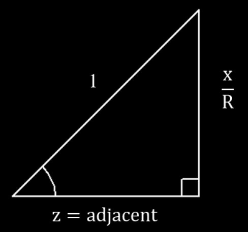
Now we can simplify a couple of the terms. The cosine with an inverse cosine in it cancels out, and we can simplify the sine of an inverse cosine with the following logic. Let’s draw a representative triangle of the inverse cosine \(cos^{-1}((R-\delta)/R)\), which can be conceptualized as “what angle has a cosine equal to \((R-\delta)/R\)?”. It looks like this:
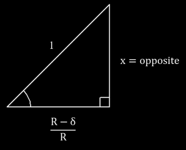
Since we now want to take the cosine of this angle, we will need to opposite side length, which I denoted as \(x\). To do this we just use the Pythagorean Theorem. This gives us:
\[sin[cos^{-1}(\frac{R-\delta}{R})] = \sqrt{1-(\frac{R-\delta}{R}^2)}\]
Which we can simplify just a bit further like so:
\[\sqrt{1-(\frac{R-\delta}{R}^2)} \\[0.5em]
= \sqrt{1-(\frac{R^2}{R^2}-\frac{2R\delta}{R^2}+\frac{\delta^2}{R^2})} \\[0.5em]
= \sqrt{\frac{2R\delta}{R^2}-\frac{\delta^2}{R^2}} \\[0.5em]
= \frac{1}{R}\sqrt{2R\delta-\delta^2}\]
Putting those simplified terms back in our \(A_{segment}\) formula finally gives the formula we will use for the segment area.
\[A_{segment} = R^2cos^{-1}(\frac{R-\delta}{R})-R^2(\frac{R-\delta}{R}*\frac{1}{R}\sqrt{2R\delta-\delta^2}) \\[0.5em]
= R^2cos^{-1}(\frac{R-\delta}{R})-(R-\delta)\sqrt{2R\delta-\delta^2} \tag{3}\]
Segment Centroid Derivation
Now we will need the centroid of a circular segment based on its depth, \(\delta\). We can approach this with calculus, using an equation for a quarter of the circle that looks like this:
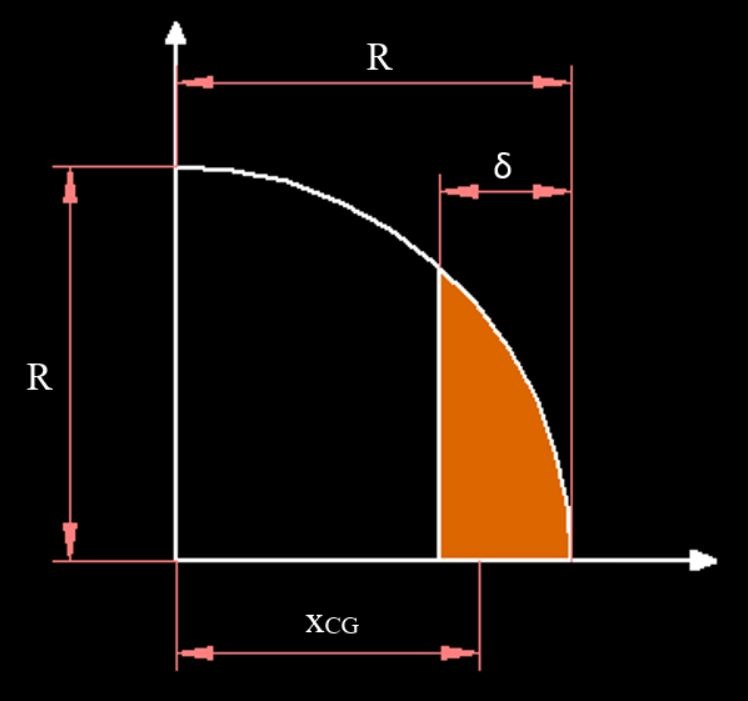
Through symmetry, we know that the centroid of this half of the circular segment is the same as the centroid for the whole segment. The equation for a circle is shown below, which we then put in terms of y.
\[R^2 = x^2+y^2 \\[0.5em]
y = \sqrt{R^2-x^2}\]
The general formula for finding a centroid through integration is shown below.
\[\bar{x} = \frac{\int_a^bxf(x)dx}{\int_a^bf(x)dx}\]
Where the denominator is just equal to the area under the curve. In our case it looks like this.
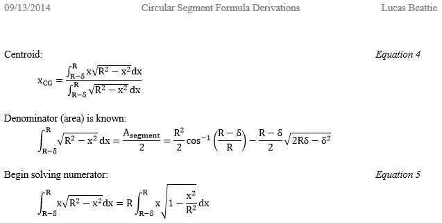
\[\bar{x} = \frac{\int_{R-\delta}^Rx\sqrt{R^2-x^2}dx}{\int_{R-\delta}^R\sqrt{R^2-x^2}dx} \tag{4}\]
Fortunately, the denominator is equal to one-half of the total segment area and is already known from Eqn. 3 above.
\[\int_{R-\delta}^R\sqrt{R^2-x^2}dx \\[0.5em]
= \frac{1}{2}(R^2cos^{-1}(\frac{R-\delta}{R})-(R-\delta)\sqrt{2r\delta-\delta^2})\]
Now we can put our attention toward integrating the numerator.
\[\int_{R-\delta}^Rx\sqrt{R^2-x^2}dx = R\int_{R-\delta}^Rx\sqrt{1-\frac{x^2}{R^2}}dx \tag{5}\]
Yikes. Now it’s time to dust off some trigonometric substitution from back in Calculus 2. We will use the substitution:
\[\frac{x^2}{R^2} = sin^2(t)\]
Solving for x and t:
\[x = Rsin(t) \\[0.5em]
t = sin^{-1}(\frac{x}{R})\]
Now we take the derivative of \(x\) so that we can find what dx equals.
\[\frac{dx}{dt} = Rcos(t) \\[0.5em]
dx = Rcos(t)dt\]
Now we substitute those results into Eqn. 5, and I will switch to using an indefinite integral for notation.
\[R\int{x}\sqrt{1-\frac{x^2}{R^2}}dx = R\int{R}sin(t)\sqrt{1-sin^2(t)}Rcos(t)dt\]
We can simplify using the common trig identity:
\[\sqrt{1-sin^2(t)} = cos(t)\]
Which gives us:
\[R\int{x}\sqrt{1-\frac{x^2}{R^2}}dx = R^3\int{}sin(t)cos^2(t)dt \tag{6}\]
We’re not done yet! We’re going to use u substitution to finish this integral out. Two Calculus 2 techniques in one problem.
\[u = cos(t) \\[0.5em]
\frac{du}{dt} = -sin(t) \\[0.5em]
dt = \frac{-du}{sin(t)}\]
Which gives us:
\[R^3\int{}sin(t)cos^2(t)dt = R^3\int{}-u^2du\]
There we go. Now that’s a problem we can solve.
\[R^3\int{}-u^2du = R^3(-\frac{u^3}{3}+c_1)\]
Resubstituting from u substitution:
\[R^3(-\frac{u^3}{3}+c_1) = -\frac{R^3}{3}cos^3(t)+c_2\]
And resubstituting from trigonometric substitution:
\[-\frac{R^3}{3}cos^3(t)+c_2 = -\frac{R^3}{3}cos^3[sin^{-1}(\frac{x}{R})]+c_3\]
We can simplify the \(cos^3(sin^{-1}(x/R))\) term similarly to when we drew an example triangle while calculating the segment area formula. We take this following representative triangle and do the Pythagorean Theorem to get the missing side length.
\[cos^3[sin^{-1}(\frac{x}{R})] = (1-\frac{x^2}{R^2})^{3/2}\]
This gives us the indefinite solution of our original numerator in Eqn. 4.
\[\int{}x\sqrt{R^2-x^2}dx = -\frac{R^3}{3}(1-\frac{x^2}{R^2})^{3/2}+c_3 \\[0.5em]
= -\frac{1}{3}(R^2-x^2)^{3/2}+c_3\]
Now we plug the bounds of our definite integral into the equation above, which allows us to ignore the integrations constant \(c_3\):
\[\int_{R-\delta}^Rx\sqrt{R^2-x^2}dx = -\frac{1}{3}(R^2-R^2)^{3/2}+\frac{1}{3}(R^2-(R-\delta)^2)^{3/2} \\[0.5em]
= 0+\frac{1}{3}(R^2-(R^2-2R\delta+\delta^2))^{3/2} = \frac{1}{3}(2R\delta-\delta^2)^{3/2}\]
Now that we finally have our numerator, we can plug it back into the complete centroid equation, Eqn. 4.
\[\bar{x} = \frac{\int_{R-\delta}^Rx\sqrt{R^2-x^2}dx}{\int_{R-\delta}^R\sqrt{R^2-x^2}dx} = \\[0.5em]
= \frac{2(2R\delta-\delta^2)^{3/2}}{3[R^2cos^{-1}(\frac{R-\delta}{R})-(R-\delta)\sqrt{2R\delta-\delta^2}]} \\[0.5em]
= \frac{2(2R\delta-\delta^2)^{3/2}}{3A_{segment}} \tag{7}\]
We finally did it! Equations 3 and 7 give us what we need to tackle this PM diagram. If anyone sees how to simplify either of these further, definitely let me know.
Example Problem
Now I will work through one PM point on one example problem to demonstrate how to use the equations we derived. Here is the cross-section we will use:

We will analyze it at balanced condition, so where \(\epsilon_s = \epsilon_y = f_y/E_s\). Here is the stress, strain, and resultant force diagrams for it.

First we will need to know the vertical locations of the center of each of the rows of rebar. This can be determined using trigonometry. For example, if we take the center of the cross-section to be the origin, and the y-axis to be vertical with upwards being positive, we have one row at y = 0, and the location of the next row above that can be calculated like so:
\[\text{Number of Spaces} = \text{Number of Bars} = 10 \\[0.5em]
\text{Interior Angle} = 360°/\text{Number of Spaces} = 36° \\[0.5em]
sin(36°) = y/\text{Radius} \\[0.5em]
y = \text{Radius}*sin(36°) \\[0.5em]
\text{Radius} = 1/2*\text{Diameter} - \text{Clear Cover} - 1/2*\text{Rebar Diameter} = 14.44" \\[0.5em]
y = 8.49"\]
Here is a table of the results for all of the rows:
| Row |
y (in) |
| 1 |
13.73 |
| 2 |
8.49 |
| 3 |
0.00 |
| 4 |
-8.49 |
| 5 |
-13.73 |
Note that we don’t place a bar in the center of the horizontal axis. This is to minimize the depth to the most extreme rebar, which is conservative. From the table of rebar locations above, we can see that our d value is:
\[d = 1/2*\text{Diameter} - y_5 \\[0.5em]
= 18"+13.73" = 31.73"\]
Now that we have d, we can again calculate the depth to the neutral axis, c, directly.
\[c = (\frac{ε_{cu}}{ε_{cu}+ε_s})*d \\[0.5em]
= (\frac{0.003}{0.003+60ksi/29,000ksi})*31.73" = 18.8"\]
Next we calculate the strain values at each rebar row just by linearly interpolating between the neutral axis the extreme concrete compression fiber or the bottom row of steel.
We then take these values and calculate stresses. Because we assume an elastic perfectly plastic stress-strain relationship for the rebar, this means if strain in the steel is less the yield strain (\(\epsilon_y = f_y/E_s\)), then the stress is linearly interpolated between zero and yield stress (\(f_s = (\epsilon_s/\epsilon_y)*f_y\)), and if the strain in the steel is anywhere at or above the yield strain, then the stress is equal to the yield stress, \(f_y\).
Finally, we can then get the resultant forces in the steel by multiplying the stresses by the total area of steel in that row. Here is a table of strains, stresses, and resultant forces for the steel in our example problem, with compression being negative.
| Row |
Strains(in/in) |
Stresses (ksi) |
No. bars |
Forces (kip) |
| 1 |
-0.00232 |
-60.0 |
2 |
-120 |
| 2 |
-0.00148 |
-42.9 |
2 |
-85.8 |
| 3 |
-0.00012 |
-3.61 |
2 |
-7.21 |
| 4 |
0.00123 |
35.7 |
2 |
71.4 |
| 5 |
0.00207 |
60.0 |
2 |
120 |
The last force we need to calculate is that of the concrete compression block. This is what we did all that work for earlier in the article. The resultant of the force is found using Eqn. 3 with \(\delta={\beta}'c\) to find the area of the block, and multiplying it by \(0.85*f'_c\), which is the magnitude (thickness) of the block.
\[A = R^2cos^{-1}(\frac{R-\delta}{R})-(R-\delta)\sqrt{2R\delta-\delta^2} \\[0.5em]
R = 18" \\[0.5em]
\delta = {\beta}'c = 0.85*18.8" = 16.0" \\[0.5em]
A = (18")^2cos^{-1}(\frac{18"-16"}{18"}-(18"-16")\sqrt{2*18"*16"-(16")^2} \\[0.5em]
A = 436in^2 \\[0.5em]
C_{conc} = 436in^2*0.85*4ksi = 1,481kips\]
Now we need the centroid of that force, which we will calculate using Eqn. 7:
\[y_{conc} = \frac{2(2R\delta-\delta^2)^{3/2}}{3A_{segment}} \\[0.5em]
= \frac{2(2*18"*16"-(16")^2)^{3/2}}{3(436in^2)} = 8.75"\]
We finally have all of the force magnitudes and centroids! Now we sum forces to get our \(P_n\) value and sum moments about the mid-height of the section to get our \(M_n\). Here’s a table showing those results for our example problem.
| Description |
y (in) |
Forces (kip) |
Moments (kip*ft) |
| Concrete |
8.75 |
-1,481 |
1,080 |
| Steel_1 |
13.7 |
-120 |
137 |
| Steel_2 |
8.49 |
-85.8 |
60.7 |
| Steel_3 |
0 |
-7.21 |
0 |
| Steel_4 |
-8.49 |
71.4 |
50.5 |
| Steel_5 |
-13.7 |
120 |
137 |
| |
sum = |
-1,503 |
1,466 |
Summary Table & Conclusion
Here is a table showing the remaining points I calculated for our example problem, but with the sign convention for axial force flipped so that compression is positive, and a graph of the resulting nominal PM capacity curve.
| Description |
P (kip) |
M (kip*ft) |
| compression |
4,026 |
0 |
| 0εsy |
3,125 |
920 |
| 0.25εsy |
2,600 |
1,225 |
| 0.50εsy |
2,165 |
1,374 |
| 0.75εsy |
1,806 |
1,441 |
| 1εsy |
1,503 |
1,466 |
| 2εsy |
801 |
1,275 |
| 3εsy |
410 |
1,047 |
| 4εsy |
194 |
867 |
| 6εsy |
-88 |
604 |
| 8εsy |
-237 |
448 |
| 10εsy |
-324 |
346 |
| tension |
-600 |
0 |
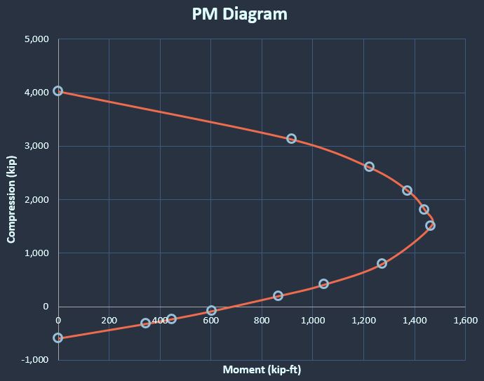
Great job making it to the end! We now can make nominal PM diagrams for circular beam-columns. In the next article we’ll wrap things up and apply phi factors, so that our results are factored and usable. We’ll also compare the results to SpColumn to see how it measures up to a more precise concrete compression block shape. And of course, I will have an Excel sheet ready to download so you can generate these curves with ease!