This is the first of a type of article I’m calling “Engineering Deep Dive.” In an engineering deep dive, I’m going to take a structural engineering problem which I found interesting to solve, and walk through it step-by-step, showing as much math as I can manage.
I expect this first deep dive topic to take about three articles, and it will cover the math behind creating a strength capacity calculator for rectangular and circular columns or drilled shafts, which are subjected to both axial load and bending moments. This type of member is called a beam-column. At the end of the series, an excel file that performs these calculations will be available for download.

The three articles will be organized like so.
- Part 1 - Nominal capacity curve for rectangular cross-sections
- Part 2 - Nominal capacity curve for circular cross-sections
- Part 3 - Phi factor application and sheet download
Background
Those who have been brave enough to read on probably already know this, but I’ll give a quick background on reinforced concrete. Concrete is cheap and is extremely strong in compression (being squished), but it is very weak in tension (being pulled apart). This is why it’s reinforced with steel reinforcing bars, which are strong in tension. These two types of loads which act longitudinally on the member are called axial loads.
When subjected to bending (imagine breaking a stick over your knee), the member experiences a combination of compression and tension. Because of this, a reinforced concrete member can actually handle more bending if it also has a bit of extra compression loading on it.
The capacity we will calculate will be in the form of a graph of a curve showing the points of theoretical failure at different combinations of axial loads. This is commonly called a PM diagram, as P is a variable commonly used to represent axial loads, and M is often used for bending moment loads.
From here on, I assume the reader has a working knowledge of structural engineering concepts. So my non-engineer friends should read onwards at their own risk!
Assumptions
I’m a bridge engineer, so I will make this calculator complaint with the AASHTO LRFD Bridge Design Specifications, 9th Edition. These concepts and the final result should match up reasonably well with the ACI code for my buildings-focused engineering friends. If you walk through these articles with me, doing the math for ACI factors and assumptions would be straightforward.
Here are some of the assumptions we will use in developing this calculator. These are either required or allowed by AASHTO section 5.6.2.
- Strain compatibility - plane sections remain plane, reinforcement is fully developed and bonded, and strain is directly proportional to distance from the neutral axis.
- Maximum usable concrete compressive strain is 0.003.
- Elastic perfectly plastic steel reinforcement stress-strain relationship.
- Concrete tensile strength is neglected.
- Rectangular compressive stress distribution assumed for strength limit state for concrete (Whitney stress block).
- Concrete strength is less than or equal to 10 ksi.
- Reinforcing steel yield strength is less than or equal to 100 ksi.
- AASHTO compression-controlled vs. tension-controlled strain limits used to calculate phi factors.
We will ignore compression steel for the hand calculation examples below, but as we will discuss in part 2, when creating an Excel sheet or another program to do these calculations, it is easy to include the effect of the compression steel. So it will be included in the program provided in part 3.
We will generate the math and equations needed for the PM diagram with generalized variables, and then we will also show the math with the following example cross section.

With:
- \(f'c = 4\) ksi
- \(f_y = 60\) ksi
- \(E_s = 29,000\) ksi
Axial-Only Capacities
We’ll start off with the easiest cases: pure compression and pure tension. We will do pure tension first, and I was tought to always draw out my cross-sectional strain, stress, and resultant force diagrams when doing any reinforced concrete analysis (thanks Dr. Harik!), and while they probably aren’t needed for these purely axial cases, I will provide them for completeness.

As the concrete will be cracked in ultimate tension, the nominal strength of the section in tension is simply the tensile capacity of the rebar, which equals \(A_s*f_y\). For our example cross section the calculation is as follows.
\[P_{nt} = (A_{s\_top}+A_{s\_bot})*f_y \\[0.5em]
= (1.24in^2+1.24in^2)*60ksi = 149kips\]
And so for our PM diagram we will have the y-axis indicating axial load and the x-axis indicating moment. We will take compression to be positive y direction and tension to be negative y direction, and we will only calculate positive moments. So our first point on our nominal capacity curve is x=0, y=-149kips.
For the full compression case, you could just neglect the reinforcment (and we will be ignoring compression reinforcement in all other cases), but I went ahead and included it because it’s simple to do so. The maximum usable compression stress in concrete with f’c < 10 ksi is \(0.85*f'c\) according to AASHTO.

\[P_{nc} = 0.85*f'c*(A_g-A_s)+f_y*A_s \\[0.5em]
= 0.85*4ksi*(12in*16in-2.48in^2)+2.48in^2*60ksi = 793kips\]
Making our second point x=0, y = 793kips.
Balanced Condition
Now we’ll get more into the meat of the problem. Essentially when we make a PM diagram, we set the extreme concrete compression fiber to it’s maximum value (we are using 0.003), as this is necessary for strength failure. We then vary the strain in the reinforcing steel, and back out what combination of axial load and moment gives us that failure condition.
We can do that for as many points as we deem necessary in order to construct a decent PM curve. I prefer to choose the steel strain values by select multiples of the steel strain at first yield (\(ε_{sy}\)), which is equal to \(f_y/E_s\).
When the member fails at \(ε_s = 1.0*ε_{sy}\), this failure condition is commonly known as the balanced failure point, because if the steel strain at failure is less than this value, the concrete fails before the steel yields (compression-controlled - a sudden failure), and if the steel strain is greater than this value, the steel will yield before the section fails (tension-controlled - a slow, observable failure).
AASHTO actually sets a range of values to denote whether a section is tension or compression controlled, with an in-between zone, but we will go over that in the third article in this series.
When designing pure bending members, we want to be sure we are tension-controlled by making sure we don’t use too much rebar, so that a failure would be slow and people would see it before anything collapsed. In beam-columns, this doesn’t apply, as columns are usually compression-controlled by nature. However, the balanced condition gives us the point of greatest bending capacity to calculate for our PM diagram.

Because we know the value of the strain at the extreme compression fiber of the concrete and in the location of the rebar (which we just treat as infinitely thin at the location of the center of the reinforcement layer), we can calculate the depth of the nuetral axis, c, directly.
\[c = (\frac{ε_{cu}}{ε_{cu}+ε_s})*d \\[0.5em]
= (\frac{0.003}{0.003+60ksi/29,000ksi})*13" = 7.69"\]
And now we will calculate the resultant forces C and T. Our ß’ is 0.85 when f’c is 4ksi.
\[C = 0.85*f'c*ß'*c*b_w = 0.85*4ksi*0.85*7.69"*12" = 267kips \\[0.5em]
T=A_{s\_bot}*f_y = 1.24in^2*60ksi = 74.4kips\]
And finally, we back out \(P_n\) by subtracting T from C, and back out \(M_n\) by summing moments about a point at the centroid of the beam.
\[P_{nb} = C-T = 267kips-74.4kips = 192kips \\[0.5em]
M_{nb} = T*(d-h/2)+C*(h/2-ß'*c/2) \\[0.5em]
= 74.4kips*(13"-8")+267kips*(8"-0.85*7.69"/2) = 1635kipin = 136kipft\]
We now have our 3rd point on the curve at x = 136kipft, y = 192kip.
Remaining Points
Now we simply repeat that process for as many steel reinforcement strain values as we desire. I will include the diagrams for and the resulting \(P_n\) and \(M_n\) values for \(ε_s = 0.5*ε_{sy}\) and \(ε_s = 4*ε_{sy}\), and then just the values for the remaining data points I calculated.

\[P_n = 298kips \\[0.5em]
M_n = 124kipft\]

\[P_n = 45.5kips \\[0.5em]
M_n = 96.3kipft\]
Summary Table
| Description |
P (kip) |
M (kip*ft) |
| compression |
793 |
0.0 |
| 0εsy |
451 |
93.0 |
| 0.25εsy |
366 |
113 |
| 0.5εsy |
298 |
124 |
| 0.75εsy |
241 |
131 |
| 1εsy |
192 |
136 |
| 2εsy |
115 |
121 |
| 3εsy |
72.5 |
107 |
| 4εsy |
45.5 |
96.3 |
| 6εsy |
13.3 |
81.6 |
| 8εsy |
-5.2 |
72.2 |
| 10εsy |
-17.3 |
65.7 |
| tension |
-74.4 |
0.0 |
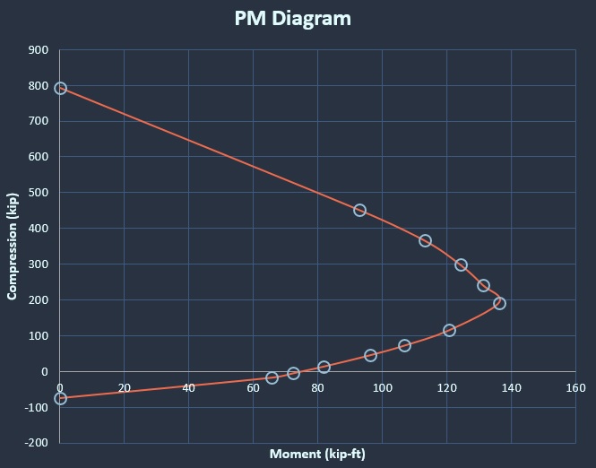
Conclusion
Now we can make nominal PM diagrams for rectangular beam-columns! I’ll show a graph of the result below. Thanks for reading and I hope it’s been helpful. In the next article we’ll begin thinking about doing the same thing for a circular section.