I hope my last VBA post left you champing at the bit to learn VBA and level up to a full Excel wizard. But maybe you aren’t sure where to start. Well don’t worry, this post is for you. Not only will I discuss general tips and resources for learning, but we’re also going to make your first macro! Let’s get straight to the good stuff first, and we’ll discuss continued learning at the end.
Sample Project: Moving Load Calculator
I often come across situations where someone has created a nice, complicated Excel calculator, and a slew of different cases need to be input into that calculator and the results copied out. VBA makes this painless, and we’re going to make a macro to demonstrate.
Overview
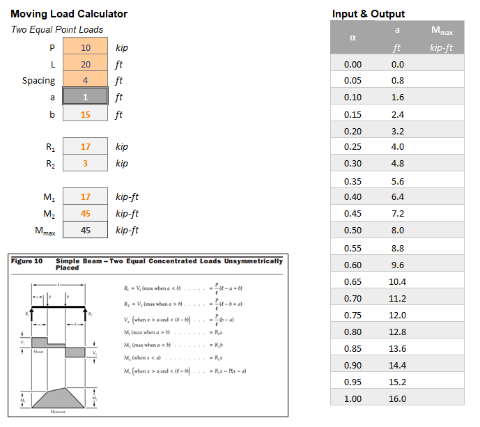
The screenshot above is a little moment calculator for a simply supported beam with two equal point loads placed on it. This sheet, without the VBA code (you’ll have to read the rest of the article and get that in yourself :P) can be downloaded here: Moving Load Calculator. But feel free to make your own from scratch if desired. If you make your own, at some point you will need to save the file as a macro-enabled file (.xlsm) just by using File, Save As.
Note that the formulas used, as well as the screenshot within the Excel file were found using American Wood Council’s Design Aid 6, available here: Design Aid 6. That’s a handy link I use frequently for shear and moment formulas.
For any non-engineers, “moment” is how much a given loading scheme is trying to bend a beam. So we would check that number versus how much bending a given beam can withstand. For the purposes of this article, I’m using a 20-ft long beam, 10-kip loads (10,000-lbs), and a 4-ft space between the loads.
Can you guess where to place the loads to generate the greatest moment demand? I’ve heard several people guess that centering the loads in the middle of the span is the worst location (ie a = 8-ft in this case). Let’s see if that’s true.
We’re going to attack this problem by inputting a large number of values of “a” and seeing what the results are. In my sheet that I linked above, I stepped “a” in increments of 0.8 feet, but any step value or inputs could be used. Note that if you use a value for “a” such that one or both of the loads fall outside the length of the beam, the results will be incorrect.
But ok, so what now? We definitely aren’t going to input each value of “a” into the calculator and copy out the results. Not when Excel has VBA for us to use! Let’s make a macro.
Making the Macro
If you do not have the “Developer” tab available in the ribbon at the top of your Excel sheet, we need to enable it. Click File, Options, Customize Ribbon (on the left sidebar), and on the right side of the screen, make sure “Developer” is checked. Now it will be on the ribbon.
Now open up the VBA edit by clicking Developer, Visual Basic (far left). To start a new macro, click Insert, Module. Now click into the editor space to begin typing.
The type of module we are going to make is called a subroutine. To initiate it, type “sub moving_load()” and press enter. Note that you can’t have spaces in the name of a subroutine, which is why we use an underscore. Now the code on your screen should look like this:
Sub moving_load()

End Sub
Excel is nice enough to go ahead and put the syntax needed to end the subroutine at the bottom for you. You can click in between the two lines and press enter a few times to give yourself more room to type.
Now we are going to define our first variable, which will describe the number of the current row we want the macro to refer to. I will call it “rw”. Since the inputs for the value of “a” that we want to put into the calculator begin in cell J5, we will start by defining rw as the value 5. To do that, simply type “rw=5” within the bounds of your sub routine. Excel will take care of adding the proper spaces for you when you click outside that line.
Next, we are going to discuss how you refer to cells in Excel while using VBA. There are two primary ways to do so, first is by using the Range() object, and second is by using the Cells() object. Anything can be done using either one, so neither one is better than the other. However, Cells() is more convenient when you want to use a variable to reference a cell, and Range() is a bit more clear when you always want to reference the same cell/cells.
For the next line, let’s type
Range("c7").Value = Cells(rw, 10).Value
When using the range object, you just reference the cell(s) as Excel would, with a letter for the column and a number for the row, but they must always be inside quotation marks. When using the cells object, you give it first the number of the row you want to reference, then a comma, then the number of the column you want to reference. In this case we want to reference the row number that our rw variable indicates (5 for now), and the column will always be column number 10 (corresponds to column J).
This line of code sets cells C7 equal to our first input for “a”, which is 0.0-ft and is found in cell J5. Can you guess what the next step will be? We want to pull out the maximum moment, and get it into cell K5. Give it a try and see if you can get that line figured out before reading ahead. I’ll wait…
Ok! We will accomplish that with this line of code:
Cells(rw, 11).Value = Range("c15").Value
If you used the cells object when I used the range object or vice versa, then it was still excellent work. However, we will want it as shown above before moving on. The reason is that the left side of the equation will reference different cells as we work our way down the chart, changing the rw variable, whereas the maximum moment output will always be located in cell C15. So now your code should look like this:
sub moving_load()
rw = 5

Range("c7").Value = Cells(rw, 10).Value
Cells(rw, 11).Value = Range("c15").Value

End Sub
And if you haven’t tried to run it yet, you should give it try! Also it’s good advice to ALWAYS save your file before running an untested macro.
To run your macro, you have a few options.
- You can click anywhere inside the code of the subroutine and click Run, Run Sub/Userform.
- F5 is the shortcut key to do the same thing.
- You can click Developer, Macros, select moving_load, and click Run.
- You can create a button to click to run the macro, which we will go over at the end of this project.
As you no doubt see, this just gets our very first input into the calculator and takes our very first output out. Not too impressive yet. So now we’re really going to spice things up with a loop. A loop is common in programming, and does a certain action a certain number of times. We’re going to use a “while loop” in this project.
In a line between your rw assignment and your C7 range assignment, type:
do while cells(rw,10).value <> ""
This is the beginning of a loop, and I will explain it shortly, but first, I recommend always closing any loop as soon as you type out the start of it. To do that, in a line just before “End Sub”, type “loop”. Lastly, it’s good style to indent within a loop, so we will select our two lines within the loop by highlighting some of both lines, and pressing “tab”.
Ok now we will go over what we typed to start this loop. You might be able to work through it just by sight. “” means a cell is empty in VBA, so this loop says it will do whatever is inside the loop until the cell located at row “rw” and column 10 is empty.
So are we done? Not quite yet. As you might imagine, since we currently never change the value of rw and we never delete our “a” input in cell J5, this loop would run forever. What we really want is to work our way down the input chart until the end of it, which we can do by increasing the value of rw by 1 each time. To accomplish this we simply add “rw=rw+1” above the line with “Loop”. Now finally, your code should look like this:
Sub moving_load()

rw = 5

Do While Cells(rw, 10).Value <> ""
    Range("c7").Value = Cells(rw, 10).Value
    Cells(rw, 11).Value = Range("c15").Value

    rw = rw + 1
Loop

End Sub
So to recap, this code sets rw to the value of 5 (the row where our inputs start). It then goes into a loop that will run until it reaches the end of our inputs. It puts our input into cell C7, and pulls the maximum moment out of cell C15. And that’s it! You’ve done it.
Now if you run it you get results! And we can see that a = 8 was NOT the worst location for moment demand. Many older engineers who know a lot of rules of thumb probably already knew that. But if that surprised you, I recommend creating a finer discretization (smaller step size) and finding out where the worst location is.
Congratulations, you made your first macro! As a final tip, when you reopen this file later, or when you send it to a coworker, you have to click “Enable Content” at the top of the page to allow excel to run macros.
General Tips
Now that you’re riding high on your major success, I will go over how I might recommend continued learning. There are a great number of free resources out there to help you learn. The one that I used probably 10 years ago and that I still recommend is WiseOwl tutorials on YouTube. The playlist can be found here: Excel VBA Introduction.
Don’t get scared off by the more than 100 videos. I would recommend watching and working along through part 25 (arrays) at most. After that just skip around and watch any topics that sound interesting. But really, by then, you are more than equipped to do your own projects, just googling for solutions to questions you have along the way.
Also, with this and any other VBA resource, you should work alongside the videos, and I encourage you to do your own projects as soon as you have the tools to do so. This is not the type of thing where you must finish studying before trying it out for yourself. Get your hands dirty as soon as possible and learn more as you go!
Nobody wants to have to go through the arduous process of clicking Developer, Macros to access their macro. What a drag! Let alone explaining to a coworker how to do that if they use your sheet. We need a button!
There are a few ways to make a button, but I’ll quickly teach you my favorite. In Excel, click Insert, Shapes, and then click the rectangle with rounded corners. You can use any shape for this, but that’s a good looking one. Now draw it in where you want your button to be. You can move and resize it later (tip: hold alt while moving it to align it with cells).
Type in whatever you want your button to say, then click out of it anywhere on the sheet. Then click it again to select it, and click Home at the top of the ribbon. Center your text horizontally and vertically to make it look better. Now click Format in the ribbon. Here you can adjust shape fill color, shape outline color, and shape outline weight to customize your button and make it look nice.
Finally right-click your button and click Assign Macro. Select your macro and click OK. Now you can run your macro by clicking the button.