Ever wondered where those concrete working stress formulas with \(\rho\), \(j\), and \(k\) come from? It seems like everybody has them in some old spreadsheet or a MacGregor textbook, but I always wondered how to get them. Should be able to get there from strain compatibility right? Let’s do it.
In bridge design these days, we almost exclusive use the Whitney stress block for dealing with concrete’s stress-strain relationship (at least before booting up some software), which works well for the strength limit state. However, the crack control equations for reinforced concrete in chapter 5 still require calculating \(f{ss}\), the stress in the reinforcement at the service limit state. It feels like all engineers have some reference to these formulas to solve it, likely just written into a spreadsheet from the previous job.
\[k = \sqrt{2\rho n + (\rho n)^2 - \rho n} \tag{1}\]
\[j = 1 - k/3 \tag{2}\]
\[f_{ss} = M_s / ( A_sjd) \tag{3}\]
These equations assume that, at service load, the concrete stress-strain relationship (as well as the rebar steel) is linear. This used to be how concrete was designed and analyzed and was called Working Stress Design (WSD). They give us a way to go from the known applied service moment (\(M_s\)) and get the associated stress in the rebar (\(f_{ss}\)).
I wanted to know where these formulas came from. I don’t see that they’re mentioned in AASHTO, and a quick flip through the MacGregor textbook showed the formulas, but show little to nothing on where they came from. I mean they used to use WSD all the time to design concrete right? Can’t be too hard.
I knew I had solved the same problem iteratively through strain compatibility in the past, so I figured I’d start there, and drew out the trusty strain, stress, force diagrams.
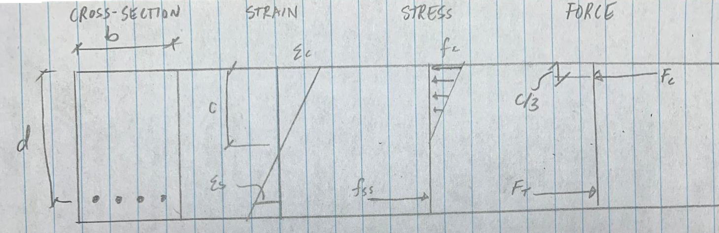
I’ve been out of practice writing articles for too long to bother making some fancy graphics, so hand sketch it is. We can see by the diagram that \(F_C\), the resultant compression force can be written as:
\[F_C = f_cbc/2\]
Putting that in terms of strain (\(f_c = E_c\epsilon_c\)) gives us Equation 4.
\[F_C = \epsilon_cE_cbc/2 \tag{4}\]
We’ll use similar triangles and our linear strain diagram to relate \(\epsilon_c\) to \(\epsilon_s\) in equation 5.
\[\epsilon_c = (\frac{c}{d-c})\epsilon_s \tag{5}\]
For static equilibrium, the sum of horizontal forces is zero, we can set \(F_T\) equal to \(F_C\), and we can substitute Equation 5 into Equation 4.
\[F_T = \frac{\epsilon_cE_cbc}{2} = \frac{c^2\epsilon_sE_cb}{2(d-c)}\]
Using steel’s linear stress-strain relationship gives us:
\[\epsilon_s = f_s / E_s = F_T/(E_sA_s)\]
Substituting that in gives:
\[F_T = \frac{F_TE_cbc^2}{2A_sE_s(d-c)}\]
\[1 = \frac{E_cbc^2}{2A_sE_s(d-c)}\]
Our unknown here is \(c\), and that looks like something that can be solved with a little quadratic formula work.
\[2A_sE_s(d-c) = E_cbc^2\]
\[E_cbc^2 + 2A_sE_sc - 2A_sE_sd=0\]
\[x=\frac{-b\pm\sqrt{b^2-4ac}}{2a}\]
\[c=\frac{-2A_sE_s+\sqrt{(2A_sE_s)^2-4E_cb(-2A_sE_sd)}}{2E_cb}\]
\[c=\frac{-2A_sE_s+\sqrt{4A_s^2E_s^2+8E_cbA_sE_sd}}{2E_cb}\]
Now separating the terms, and pulling a 2 from inside the square root gives us:
\[c=\frac{\sqrt{A_s^2E_s^2+2E_cbA_sE_sd}}{E_cb}-\frac{A_sE_s}{E_cb}\]
Ok here’s about where I expected to flounder. How do we get from here to those nice compact k and j equations? I don’t know who came up with the idea to use the modular ratio (\(n\)) in these, or if there’s a more intuitive way to think about it that makes it obvious, but I know we need to move toward getting things in terms of \(n\), so let’s move toward \(E_s / E_c\) where possible
\[c=\sqrt{\frac{A_s^2E_s^2}{E_c^2b^2}+\frac{2E_cbA_sE_sd}{E_c^2b^2}}-\frac{A_sE_s}{E_cb}\]
\[c=\sqrt{\frac{A_s^2}{b^2}\frac{E_s^2}{E_c^2}+2\frac{E_s}{E_c}\frac{A_sd}{b}}-\frac{A_s}{b}\frac{E_s}{E_c}\]
\[n = \frac{E_s}{E_c}\]
\[c=\sqrt{n^2\frac{A_s^2}{b^2}+2n\frac{A_sd}{b}}-n\frac{A_s}{b}\]
Nice, we’re getting closer. Now for the next trick, we’ll continue to work toward the final format, and try to put things in terms of \(\rho\), the reinforcement ratio.
\[\rho = \frac{A_s}{bd}\]
However, you’ll see that in our equation so far, the terms are all \(A_s/b\), so we need an extra \(d\). This is where inventing that \(k\) variable comes in so much use. Again, not sure who thought of that or if there’s a more obvious way to conceptualize it, but it seems like a stroke of ingenious simplicity to me.
\[c = kd\]
\[k = c/d\]
So now we just need to put a \(d\) in the denominator (or a \(d^2\) in the denominator inside a square root).
\[k = \frac{c}{d}=\sqrt{n^2\frac{A_s^2}{b^2d^2}+2n\frac{A_s}{bd}}-n\frac{A_s}{bd}\]
Viola!
\[k = \sqrt{n^2\rho^2+2n\rho}-n\rho \tag{3}\]
One of three down, and its all downhill from here. I was so satisfied when that worked out in my hand calc.
So next, we go back to our force diagram from the photo, and we take a sum of moments about the compression force centroid. In this problem, we know the applied moment and are trying to get the associated service steel stress, so the value of the sum of moments is known.
\[\Sigma M = M_s = F_T(d-c/3)\]
\[F_T = \frac{M_s}{d-c/3}\]
Now, knowing that the stress in the rebar is \(F_T/A_s\) and substituting in our \(c=kd\) from earlier:
\[f_{ss} = \frac{F_T}{A_s} = \frac{M}{A_s(d - kd/3)} = \frac{M}{A_sd(1 - k/3)}\]
We have it! You can see that the final step is creating a variable \(j\) to slightly simplify. This one seems much less useful than the \(k\), \(\rho\), and \(n\) simplifications, but for completeness:
\[j = 1 - k/3 \tag{2}\]
\[f_{ss} = M_s / (A_sjd) \tag{3}\]

We’ve done it! Always good to see those mysterious, ancient equations bequeathed to us young(ish) engineers, used to relying on our computer crutches, boil down to strain compatibility. Truly among the most useful of structural engineering assumptions. I had a good time working this out, and was really pleased when the simplifications all came together. Hope this is helpful or interesting to someone!